Writing SQL Queries for Dashboards
This guide provides practical recipes and patterns for writing useful SQL queries in Logfire. We'll focus on querying the records table, which contains your logs and spans. The goal is to help you create useful dashboards, but we recommend using the Explore view to learn and experiment.
For a complete list of available tables and columns, please see the SQL Reference.
Finding common cases
Simple examples
Here are two quick useful examples to try out immediately in the Explore view.
To find the most common operations based on span_name:
SELECT
    COUNT() AS count,
    span_name
FROM records
GROUP BY span_name
ORDER BY count DESC
Similarly, to find the most common exception_types:
SELECT
    COUNT() AS count,
    exception_type
FROM records
WHERE is_exception
GROUP BY exception_type
ORDER BY count DESC
Finally, to find the biggest traces, which may be a sign of an operation doing too many things:
SELECT
    COUNT() AS count,
    trace_id
FROM records
GROUP BY trace_id
ORDER BY count DESC
The general pattern
The basic template is:
SELECT
    COUNT() AS count,
    <columns_to_group_by>
FROM records
WHERE <filter_conditions>
GROUP BY <columns_to_group_by>
ORDER BY count DESC
LIMIT 10
- The alias
AS countallows us to refer to the count in theORDER BYclause. ORDER BY count DESCsorts the results to show the most common groups first.WHERE <filter_conditions>is optional and depends on your specific use case.LIMIT 10isn't usually needed in the Explore view, but is helpful when creating charts.<columns_to_group_by>can be one or more columns and should be the same in theSELECTandGROUP BYclauses.
Useful things to group by
span_name: this is nice and generic and shouldn't have too much variability, creating decently sized meaningful groups. It's especially good for HTTP server request spans, where it typically contains the HTTP method and route (the path template) without the specific parameters. To focus on such spans, trying filtering by the appropriateotel_scope_name, e.g.WHERE otel_scope_name = 'opentelemetry.instrumentation.fastapi'if you're usinglogfire.instrument_fastapi().exception_typehttp_response_status_codeattributes->>'...': this will depend on your specific data. Try taking a look at some relevant spans in the Live view first to see what attributes are available.- If you have a custom attribute like
attributes->>'user_id', you can group by that to see which users are most active or have the most errors. - If you're using
logfire.instrument_fastapi(), there's often useful values inside thefastapi.arguments.valuesattribute, e.g.attributes->'fastapi.arguments.values'->>'user_id'. - All web frameworks also typically capture several other potentially useful HTTP attributes. In particular if you capture headers (e.g. with
logfire.instrument_django(capture_headers=True)) then you can try e.g.attributes->>'http.request.header.host'. - For database query spans, try
attributes->>'db.statement',attributes->>'db.query.text', orattributes->>'db.query.summary'.
- If you have a custom attribute like
message- this is often very variable which may make it less useful depending on your data. But if you're using a SQL instrumentation with the Python Logfire SDK, then this contains a rough summary of the SQL query, helping to group similar queries together ifattributes->>'db.statement'orattributes->>'db.query.text'is too granular. In this case you probably want a filter such asotel_scope_name = 'opentelemetry.instrumentation.sqlalchemy'to focus on SQL queries.service_nameif you've configured multiple services. This can easily be combined with any other column.deployment_environmentif you've configured multiple environments (e.g.productionandstaging,development) and have more than one selected in the UI at the moment. Likeservice_name, this is good for combining with other columns.
Useful WHERE clauses
is_exceptionlevel >= 'error'- maybe combined with the above with eitherANDorOR, since you can have non-error exceptions and non-exception errors.level > 'info'to also find warnings and other notable records, not just errors.http_response_status_code >= 400or500to find HTTP requests that didn't go well.service_name = '...'can help a lot to make queries faster.otel_scope_name = '...'to focus on a specific (instrumentation) library, e.g.opentelemetry.instrumentation.fastapi,logfire.openai, orpydantic-ai.duration > 2to find slow spans. Replace2with your desired number of seconds.parent_span_id IS NULLto find top-level spans, i.e. the root of a trace.
Using in Dashboards
For starters:
- Create a panel in a new or existing custom (not standard) dashboard.
- Click the Type dropdown and select Table.
- Paste your query into the SQL editor.
- Give your panel a name.
- Click Apply to save it.
Tables are easy and flexible. They can handle any number of GROUP BY columns, and don't really need a LIMIT to be practical. But they're not very pretty. Try making a bar chart instead:
- Click the pencil icon to edit your panel.
- Change the Type to Bar Chart.
- Add
LIMIT 10or so at the end of your query if there are too many bars. - If you have multiple
GROUP BYcolumns, you will need to convert them to one expression by concatenating strings. Replace each,in theGROUP BYclause with|| ' - ' ||to create a single string with dashes between the values, e.g. replaceservice_name, span_namewithservice_name || ' - ' || span_name. Do this in both theSELECTandGROUP BYclauses. You can optionally add anASalias to the concatenated string in theSELECTclause, likeservice_name || ' - ' || span_name AS service_and_span, and then use that alias in theGROUP BYclause instead of repeating the concatenation. - If your grouping column happens to be a number, add
::textto it to convert it to a string so that it's recognized as a category by the chart. - Bar charts generally put the first rows in the query result at the bottom. If you want the most common items at the top, wrap the whole query in
SELECT * FROM (<original query>) ORDER BY count ASCto flip the order. Now the innerORDER BY count DESCensures that we have the most common items (before the limit is applied) and the outerORDER BY count ASCis for appearance.
For a complete example, you can replace this:
SELECT
    COUNT() AS count,
    service_name,
    span_name
FROM records
GROUP BY service_name, span_name
ORDER BY count DESC
with:
SELECT * FROM (
    SELECT
        COUNT() AS count,
        service_name || ' - ' || span_name AS service_and_span
    FROM records
    GROUP BY service_and_span
    ORDER BY count DESC
    LIMIT 10
) ORDER BY count ASC
Finally, check the Settings tab in the panel editor to tweak the appearance of your chart.
Aggregating Numerical Data
Instead of just counting rows, you can perform calculations on numerical expressions. duration is a particularly useful column for performance analysis. Tweaking our first example:
SELECT
    SUM(duration) AS total_duration_seconds,
    span_name
FROM records
WHERE duration IS NOT NULL -- Ignore logs, which have no duration
GROUP BY span_name
ORDER BY total_duration_seconds DESC
This will show you which operations take the most time overall, whether it's because they run frequently or take a long time each time.
Alternatively you could use AVG(duration) (for the mean) or MEDIAN(duration) to find which operations are slow on average, or MAX(duration) to find the worst case scenarios. See the Datafusion documentation for the full list of available aggregation functions.
Other numerical values can typically be found inside attributes and will depend on your data. LLM spans often have attributes->'gen_ai.usage.input_tokens' and attributes->'gen_ai.usage.output_tokens' which you can use to monitor costs.
Warning
SUM(attributes->'...') and other numerical aggregations will typically return an error because the database doesn't know the type of the JSON value inside attributes, so use SUM((attributes->'...')::numeric) to convert it to a number.
Percentiles
A slightly more advanced aggregation is to calculate percentiles. For example, the 95th percentile means the value below which 95% of the data falls. This is typically referred to as P95, and tells you a more 'typical' worst-case scenario while ignoring the extreme outliers found by using MAX(). P90 and P99 are also commonly used.
To calculate this requires a bit of extra syntax:
SELECT
    approx_percentile_cont(0.95) WITHIN GROUP (ORDER BY duration) as P95,
    span_name
FROM records
WHERE duration IS NOT NULL
GROUP BY span_name
ORDER BY P95 DESC
This query calculates the 95th percentile of the duration for each span_name. The general pattern is approx_percentile_cont(<percentile>) WITHIN GROUP (ORDER BY <column>) where <percentile> is a number between 0 and 1.
Time series
Create a new panel in a dashboard, and by default it will have the type Time Series Chart with a query like this:
SELECT
    time_bucket($resolution, start_timestamp) AS x,
    count() as count
FROM records
GROUP BY x
Here the time_bucket($resolution, start_timestamp) is essential. $resolution is a special variable that exists in all dashboards and adjusts automatically based on the time range. You can adjust it while viewing the dashboard using the dropdown in the top left corner. It doesn't exist in the Explore view, so you have to use a concrete interval like time_bucket('1 hour', start_timestamp) there. Tick Show rendered query in the panel editor to fill in the resolution and other variables so that you can copy the query to the Explore view.
Warning
If you're querying metrics, use recorded_timestamp instead of start_timestamp.
You can give the time bucket expression any name (x in the example above), but it must be the same in both the SELECT and GROUP BY clauses. The chart will detect that the type is a timestamp and use it as the x-axis.
You can replace the count() with any aggregation(s) you want. For example, you can show multiple levels of percentiles:
SELECT
    time_bucket($resolution, start_timestamp) AS x,
    approx_percentile_cont(0.80) WITHIN GROUP (ORDER BY duration) AS p80,
    approx_percentile_cont(0.90) WITHIN GROUP (ORDER BY duration) AS p90,
    approx_percentile_cont(0.95) WITHIN GROUP (ORDER BY duration) AS p95
FROM records
GROUP BY x
Grouping by Dimension
You can make time series charts with multiple lines (series) for the same numerical metric by grouping by a dimension. This means adding a column to the SELECT and GROUP BY clauses and then selecting it from the 'Dimension' dropdown next to the SQL editor.
Low cardinality dimensions
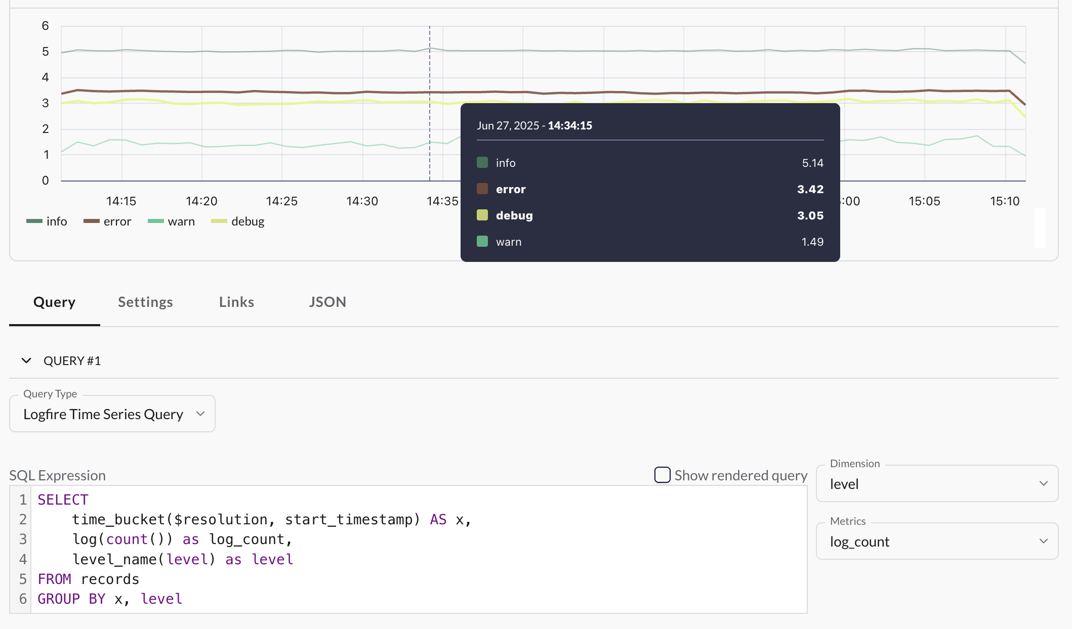
For a simple example, paste this into the SQL editor:
SELECT
    time_bucket($resolution, start_timestamp) AS x,
    log(count()) as log_count,
    level_name(level) as level
FROM records
GROUP BY x, level
Then set the Dimension dropdown to level and the Metrics dropdown to log_count. This will create a time series chart with multiple lines, one for each log level (e.g. 'info', 'warning', 'error'). Here's what the configuration and result would look like:
Note
You can only set one dimension, but you can set multiple metrics.
Here we use log(count()) instead of just count() because you probably have way more 'info' records than 'error' records, making it hard to notice any spikes in the number of errors. This compresses the y-axis into a logarithmic scale to make it more visually useful, but the numbers are harder to interpret. The level_name(level) function converts the numeric level value to a human-readable string.
You can replace level with other useful things to group by, but they need to be very low cardinality (i.e. not too many unique values) for this simple query to work well in a time series chart. Good examples are:
service_namedeployment_environmentexception_typehttp_response_status_codeattributes->>'http.method'(orattributes->>'http.request.method'for newer OpenTelemetry instrumentations)
Multiple dimensions
Because time series charts can only have one dimension, if you want to group by multiple columns, you need to concatenate them into a single string, e.g. instead of:
SELECT
    time_bucket($resolution, start_timestamp) AS x,
    log(count()) as log_count,
    service_name,
    level_name(level) as level
FROM records
GROUP BY x, service_name, level
You would do:
SELECT
    time_bucket($resolution, start_timestamp) AS x,
    log(count()) as log_count,
    service_name || ' - ' || level_name(level) AS service_and_level
FROM records
GROUP BY x, service_and_level
Then set the 'Dimension' dropdown to service_and_level. This will create a time series chart with a line for each combination of service_name and level. Of course this increases the cardinality quickly, making the next section more relevant.
High cardinality dimensions
If you try grouping by something with more than a few unique values, you'll end up with a cluttered chart with too many lines. For example, this will look like a mess unless your data is very simple:
SELECT
    time_bucket($resolution, start_timestamp) AS x,
    count() as count,
    span_name
FROM records
GROUP BY x, span_name
The quick and dirty solution is to add these lines at the end:
ORDER BY count DESC
LIMIT 200
This will give you a point for the 200 most common combinations of x and span_name. This will often work reasonably well, but the limit will need to be tuned based on the data, and the number of points at each time bucket will vary. Here's the better version:
WITH original AS (
    SELECT
        time_bucket($resolution, start_timestamp) AS x,
        count() as count,
        span_name
    FROM records
    GROUP BY x, span_name
),
ranked AS (
    SELECT
        x,
        count,
        span_name,
        ROW_NUMBER() OVER (PARTITION BY x ORDER BY count DESC) AS row_num
    FROM original
)
SELECT
    x,
    count,
    span_name
FROM ranked
WHERE row_num <= 5
ORDER BY x
This selects the top 5 span_names for each time bucket, and will usually work perfectly. It may look intimidating, but constructing a query like this can be done very mechanically. Start with a basic query in this form:
SELECT
    time_bucket($resolution, start_timestamp) AS x,
    <aggregation_expression> AS metric,
    <dimension_expression> as dimension
FROM records
GROUP BY x, dimension
Fill in <aggregation_expression> with your desired aggregation (e.g. count(), SUM(duration), etc.) and <dimension_expression> with the column(s) you want to group by (e.g. span_name). Set the 'Dimension' dropdown to dimension and the 'Metrics' dropdown to metric. That should give you a working (but probably cluttered) time series chart. Then simply paste it into <original_query> in the following template:
WITH original AS (
    <original_query>
),
ranked AS (
    SELECT
        x,
        metric,
        dimension,
        ROW_NUMBER() OVER (PARTITION BY x ORDER BY metric DESC) AS row_num
    FROM original
)
SELECT
    x,
    metric,
    dimension
FROM ranked
WHERE row_num <= 5
ORDER BY x
Linking to the Live view
While aggregating data with GROUP BY is powerful for seeing trends, sometimes you need to investigate specific events, like a single slow operation or a costly API call. In these cases, it's good to include the trace_id column in your SELECT clause. Tables in dashboards, the explore view, or alert run results with this column will render the trace_id values as clickable links to the Live View.
For example, to find the 10 slowest spans in your system, you can create a 'Table' panel with this query:
SELECT
    trace_id,
    duration,
    message
FROM records
ORDER BY duration DESC
LIMIT 10
The table alone won't tell you much, but you can click on the trace_id of any row to investigate the full context further.
You can also select the span_id column to get a link directly to a specific span within the trace viewer. However, this only works if the trace_id column is also included in your SELECT statement.
Other columns that may be useful to include in such queries:
messageis a human readable description of the span, as seen in the Live view list of records.start_timestampandend_timestampattributesservice_nameotel_scope_namedeployment_environmentotel_resource_attributesexception_typeandexception_messagehttp_response_status_codelevel_name(level)